Met Office UKV high-resolution atmosphere model data¶

Urban Sensors

Context¶

Purpose¶

To load, plot, regrid and extract an urban region from the UKV gridded model data using the Iris package.

Sensor description¶

Met Office UKV model data is fairly high resolution (approximately 1 km horizontal) and available over the whole of the UK for a variety of atmospheric variables at surface and pressure levels. A selection of variables has been made openly available as part of the Met Office contribution to the COVID 19 modelling effort. A selection of variables at hourly and daily frequency in NetCDF format can be obtained from this landing page.

This notebook uses a single sample data file for 1.5 m temperature included with the notebook.

Highlights¶

Data for the whole UK is loaded and plotted using Iris
Data is regridded to a geographic projection
A region over London is extracted

Contributions¶

Notebook¶

Samantha V. Adams (author), Met Office Informatics Lab, @svadams, 03/08/21 (latest version) Alejandro Coca-Castro (reviewer), The Alan Turing Institute, @acocac, 09/08/21 (latest revision)

Dataset originator/creator¶

Met Office Informatics Lab (creator) Microsoft (support) European Regional Development Fund (support)

Dataset authors¶

Met Office

Dataset documentation¶

Theo McCaie. Met office and partners offer data and compute platform for covid-19 researchers. URL: https://medium.com/informatics-lab/met-office-and-partners-offer-data-and-compute-platform-for-covid-19-researchers-83848ac55f5f.

Note

Note this data should be used only for non-commercial purposes.

Install and load libraries¶

#!conda install -c conda-forge iris

import iris
import iris.analysis
import iris.plot as iplt
from iris.coords import DimCoord
from iris.coord_systems import GeogCS
from iris.cube import Cube

from iris.fileformats.pp import EARTH_RADIUS

import urllib.request

import numpy as np
import matplotlib.pyplot as plt
%matplotlib     inline

Retrieve and load a sample data file¶

filepath = 'https://metdatasa.blob.core.windows.net/covid19-response-non-commercial/metoffice_ukv_daily/t1o5m_mean/'
filename = 'ukv_daily_t1o5m_mean_20150801.nc'
urllib.request.urlretrieve(filepath+filename, '../sensors/' + filename)

('../sensors/ukv_daily_t1o5m_mean_20150801.nc',
 <http.client.HTTPMessage at 0x7f89f7dd6cd0>)

air_temp = iris.load_cube('../sensors/' + filename)
air_temp.coord('grid_latitude').guess_bounds()
air_temp.coord('grid_longitude').guess_bounds()

Visualisation¶

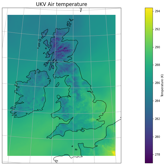
Here we use the Iris wrapper to matplotlib pyplot to plot the gridded data with added gridlines and coastline.

plt.figure(figsize=(30, 10))
iplt.pcolormesh(air_temp)
plt.title("UKV Air temperature", fontsize="xx-large")
cbar = plt.colorbar()
cbar.set_label('Temperature (' + str(air_temp.units) + ')')
ax = plt.gca()
ax.coastlines(resolution="50m")
ax.gridlines()

<cartopy.mpl.gridliner.Gridliner at 0x7f89ff071850>

Regridding from Azimuthal equal-area projection to geographic¶

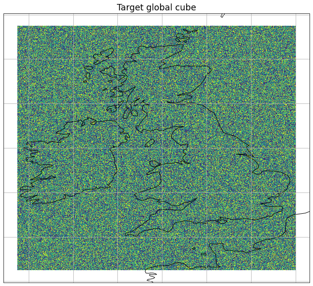
Create a target cube with a lat-lon coord system for regrid¶

It is filled with random data so we can plot it to check it looks correct.

latitude = DimCoord(np.linspace(48.5, 59.5, 1222),
                    standard_name='latitude',
                    coord_system = GeogCS(EARTH_RADIUS),
                    units='degrees')
longitude = DimCoord(np.linspace(-10.5, 2.0, 1389),
                     standard_name='longitude',
                    coord_system = GeogCS(EARTH_RADIUS),                     
                     units='degrees')
global_cube = Cube(np.random.uniform(low=0.0, high=1.0, size=(1222, 1389)),
                   dim_coords_and_dims=[(latitude, 0),
                                        (longitude, 1)])

global_cube.coord('latitude').guess_bounds()
global_cube.coord('longitude').guess_bounds()

plt.figure(figsize=(30, 10))
iplt.pcolormesh(global_cube)
plt.title("Target global cube", fontsize="xx-large")
ax = plt.gca()
ax.coastlines(resolution="50m")
ax.gridlines()

<cartopy.mpl.gridliner.Gridliner at 0x7f89fbec4c10>

../../_images/urban-sensors-ukv_12_1.png

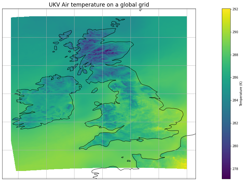
Perform the regridding from source data cube to target cube¶

# Note we need to use extrapolation masking in case regridded source data is actually smaller
# than the target cube extents
global_air_temp = air_temp.regrid(global_cube, iris.analysis.Linear(extrapolation_mode="mask"))

Plot the regridded data to check it is correct¶

plt.figure(figsize=(30, 10))

iplt.pcolormesh(global_air_temp)
plt.title("UKV Air temperature on a global grid", fontsize="xx-large")
cbar = plt.colorbar()
cbar.set_label('Temperature (' + str(global_air_temp.units) + ')')
ax = plt.gca()
ax.coastlines(resolution="50m")
ax.gridlines()

<cartopy.mpl.gridliner.Gridliner at 0x7f89fc240eb0>

../../_images/urban-sensors-ukv_16_1.png

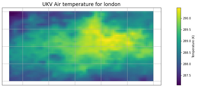
Extract the London Region¶

Use the Iris Intersection method and supply the region lat-lon bounds¶

min_lon = -0.52
min_lat = 51.3
max_lon = 0.3
max_lat = 51.7

air_temp_london = global_air_temp.intersection(longitude=(min_lon, max_lon), latitude=(min_lat, max_lat))

Plot the results¶

plt.figure(figsize=(20, 5))

iplt.pcolormesh(air_temp_london)
plt.title("UKV Air temperature for london", fontsize="xx-large")
cbar = plt.colorbar()
cbar.set_label('Temperature (' + str(air_temp_london.units) + ')')
ax = plt.gca()
ax.coastlines(resolution="50m")
ax.gridlines()

plt.show()

../../_images/urban-sensors-ukv_20_0.png

Save as a new NetCDF file¶

iris.save(air_temp_london, '../sensors/ukv_london_sample.nc')

Summary¶

This notebook has demonstrated the use of the Iris package to easily load, plot and manipulate gridded environmental NetCDF data.

Version¶

Notebook: commit 74bbb54

The Environmental AI book