Tree crown detection using DeepForest
Forest Modelling
Context
Purpose
Detect tree crown using a state-of-art Deep Learning model for object detection.
Modelling approach
A prebuilt Deep Learning model, named DeepForest, is used to predict individual tree crowns from an airborne RGB image. DeepForest was trained on data from the National Ecological Observatory Network (NEON). DeepForest was implemented in Python 3.7 using initally Tensorflow v1.14 but later moved to Pytorch. Further details can be found in the package documentation.
Highlights
Fetch and load a NEON image from a Zenodo repository using
intakeanddask.Retrieve and plot the ground-truth annotations (bounding boxes) for the target image.
Load and use a pretrained DeepForest model to generate predictions from the full-image or tile-wise prediction.
Indicate the pros and cons of full-image and tile-wise prediction.
Contributions
Notebook
Alejandro Coca-Castro (author), The Alan Turing Institute, @acocac Matt Allen (reviewer), Department of Geography - University of Cambridge, @mja2106, 21/09/21 (latest revision)
Modelling codebase
Ben Weinstein (maintainer & developer), University of Florida, @bw4sz
Henry Senyondo (support maintainer), University of Florida, @ethanwhite
Ethan White (PI and author), University of Florida, @weecology
Other contributors are listed in the GitHub repo
Modelling publications
Ben G Weinstein, Sergio Marconi, Mélaine Aubry-Kientz, Gregoire Vincent, Henry Senyondo, and Ethan P White. Deepforest: a python package for rgb deep learning tree crown delineation. Methods in Ecology and Evolution, 11:1743–1751, 2020. URL: https://besjournals.onlinelibrary.wiley.com/doi/abs/10.1111/2041-210X.13472, doi:https://doi.org/10.1111/2041-210X.13472.
Ben G Weinstein, Sergio Marconi, Stephanie Bohlman, Alina Zare, and Ethan White. Individual tree-crown detection in rgb imagery using semi-supervised deep learning neural networks. Remote Sensing, 2019. URL: https://www.mdpi.com/2072-4292/11/11/1309, doi:10.3390/rs11111309.
Ben G Weinstein, Sergio Marconi, Stephanie A Bohlman, Alina Zare, and Ethan P White. Cross-site learning in deep learning rgb tree crown detection. Ecological Informatics, 56:101061, 2020. URL: https://www.sciencedirect.com/science/article/pii/S157495412030011X, doi:https://doi.org/10.1016/j.ecoinf.2020.101061.
Modelling funding
TBD
Note
The author acknowledges DeepForest contributors. Some code snippets were extracted from DeepForest GitHub public repository.
Install and load libraries
!pip -q install git+https://github.com/ESM-VFC/intake_zenodo_fetcher.git ##Intake Zenodo Fetcher
!pip -q install pycurl
!pip -q install DeepForest
import glob
import os
import urllib
import numpy as np

import intake
from intake_zenodo_fetcher import download_zenodo_files_for_entry
import matplotlib.pyplot as plt
import xmltodict
import cv2

import tempfile

import torch

%matplotlib inline
Fetch a RGB image from Zenodo
Fetch a sample image from a publically accessible location.
# create a temp dir
path = tempfile.mkdtemp()

catalog_file = os.path.join(path, 'catalog.yaml')

with open(catalog_file, 'w') as f:
    f.write('''
sources:
  NEONTREE_rgb:
    driver: xarray_image
    description: 'NeonTreeEvaluation RGB images (collection)'
    metadata:
      zenodo_doi: "10.5281/zenodo.3459803"
    args:
      urlpath: "{{ CATALOG_DIR }}/NEONsample_RGB/2018_MLBS_3_541000_4140000_image_crop.tif"
      ''')
Load an intake catalog for the downloaded data.
cat_tc = intake.open_catalog(catalog_file)
for catalog_entry in list(cat_tc):
    download_zenodo_files_for_entry(
        cat_tc[catalog_entry],
        force_download=False
    )
will download https://zenodo.org/api/files/5b372ed9-e4ec-41b0-a652-f0ce7d760e60/2018_MLBS_3_541000_4140000_image_crop.tif to /var/folders/l8/99_59fvn4bl2szm125grkgqw0000gr/T/tmppno_cnsy/NEONsample_RGB/2018_MLBS_3_541000_4140000_image_crop.tif
Load sample image
Here we use intake to load the image through dask.
tc_rgb = cat_tc["NEONTREE_rgb"].to_dask()
/Users/acoca/anaconda3/envs/envai-book/lib/python3.8/site-packages/intake_xarray/image.py:337: FutureWarning: open_files is deprecated and will be removed in a future release. Please use fsspec.core.open_files instead.
  files = open_files(self.urlpath, **self.storage_options)
/Users/acoca/anaconda3/envs/envai-book/lib/python3.8/site-packages/xarray/core/dataset.py:2145: FutureWarning: None value for 'chunks' is deprecated. It will raise an error in the future. Use instead '{}'
  warnings.warn(
tc_rgb
<xarray.DataArray (y: 1864, x: 1429, channel: 3)>
dask.array<xarray-<this-array>, shape=(1864, 1429, 3), dtype=uint8, chunksize=(1864, 1429, 3), chunktype=numpy.ndarray>
Coordinates:
  * y        (y) int64 0 1 2 3 4 5 6 7 ... 1857 1858 1859 1860 1861 1862 1863
  * x        (x) int64 0 1 2 3 4 5 6 7 ... 1422 1423 1424 1425 1426 1427 1428
  * channel  (channel) int64 0 1 2
- y: 1864
- x: 1429
- channel: 3
- dask.array<chunksize=(1864, 1429, 3), meta=np.ndarray>
Array Chunk Bytes 7.62 MiB 7.62 MiB Shape (1864, 1429, 3) (1864, 1429, 3) Count 1 Tasks 1 Chunks Type uint8 numpy.ndarray - y(y)int640 1 2 3 4 ... 1860 1861 1862 1863
array([ 0, 1, 2, ..., 1861, 1862, 1863])
- x(x)int640 1 2 3 4 ... 1425 1426 1427 1428
array([ 0, 1, 2, ..., 1426, 1427, 1428])
- channel(channel)int640 1 2
array([0, 1, 2])
Load and prepare labels
filenames = glob.glob(os.path.join(path, './NEONsample_RGB/*.tif'))
filesn = [os.path.basename(i) for i in filenames]
##Create ordered dictionary of .xml annotation files
def loadxml(imagename):
  imagename = imagename.replace('.tif','')
  fullurl = "https://raw.githubusercontent.com/weecology/NeonTreeEvaluation/master/annotations/" + imagename + ".xml"
  file = urllib.request.urlopen(fullurl)
  data = file.read()
  file.close()
  data = xmltodict.parse(data)
  return data

allxml = [loadxml(i) for i in filesn]
# function to extract bounding boxes
def extractbb(i):
  bb = [f['bndbox'] for f in allxml[i]['annotation']['object']]
  return bb

bball = [extractbb(i) for i in range(0,len(allxml))]
print(len(bball))
1
Visualise image and labels
# function to plot images
def cv2_imshow(a, **kwargs):
    a = a.clip(0, 255).astype('uint8')
    # cv2 stores colors as BGR; convert to RGB
    if a.ndim == 3:
        if a.shape[2] == 4:
            a = cv2.cvtColor(a, cv2.COLOR_BGRA2RGBA)
        else:
            a = cv2.cvtColor(a, cv2.COLOR_BGR2RGB)

    return plt.imshow(a, **kwargs)
image = tc_rgb
# plot predicted bbox
image2 = image.values.copy()
target_bbox = bball[0]
print(type(target_bbox))
print(target_bbox[0:2])
<class 'list'>
[OrderedDict([('xmin', '1377'), ('ymin', '697'), ('xmax', '1429'), ('ymax', '752')]), OrderedDict([('xmin', '787'), ('ymin', '232'), ('xmax', '811'), ('ymax', '256')])]
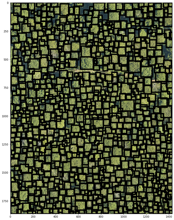
for row in target_bbox:
    cv2.rectangle(image2, (int(row["xmin"]), int(row["ymin"])), (int(row["xmax"]), int(row["ymax"])), (0, 0, 0), thickness=10, lineType=cv2.LINE_AA)

plt.figure(figsize=(15,15))
cv2_imshow(np.flip(image2,2))
plt.show()
Load DeepForest pretrained model
Now we’re going to load and use a pretrained model from the deepforest package.
from deepforest import main
# load deep forest model
model = main.deepforest()
model.use_release()
model.current_device = torch.device("cpu")
Reading config file: /Users/acoca/anaconda3/envs/envai-book/lib/python3.8/site-packages/deepforest/data/deepforest_config.yml
Model from DeepForest release https://github.com/weecology/DeepForest/releases/tag/1.0.0 was already downloaded. Loading model from file.
Loading pre-built model: https://github.com/weecology/DeepForest/releases/tag/1.0.0
pred_boxes = model.predict_image(image=image.values)
print(pred_boxes.head(5))
/Users/acoca/anaconda3/envs/envai-book/lib/python3.8/site-packages/deepforest/predict.py:32: UserWarning: Image type is {}, transforming to float32. This assumes that the range of pixel values is 0-255, as opposed to 0-1.To suppress this warning, transform image (image.astype('float32')
  warnings.warn("Image type is {}, transforming to float32. This assumes that the range of pixel values is 0-255, as opposed to 0-1.To suppress this warning, transform image (image.astype('float32')")
     xmin   ymin    xmax   ymax label     score
0  1258.0  561.0  1399.0  698.0  Tree  0.415253
1  1119.0  527.0  1255.0  660.0  Tree  0.395937
2     7.0  248.0   140.0  395.0  Tree  0.376462
3   444.0  459.0   575.0  582.0  Tree  0.355283
4    94.0  149.0   208.0  260.0  Tree  0.347175
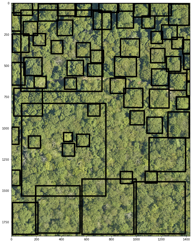
image3 = image.values.copy()

for index, row in pred_boxes.iterrows():
    cv2.rectangle(image3, (int(row["xmin"]), int(row["ymin"])), (int(row["xmax"]), int(row["ymax"])), (0, 0, 0), thickness=10, lineType=cv2.LINE_AA)

plt.figure(figsize=(15,15))
cv2_imshow(np.flip(image3,2))
plt.show()
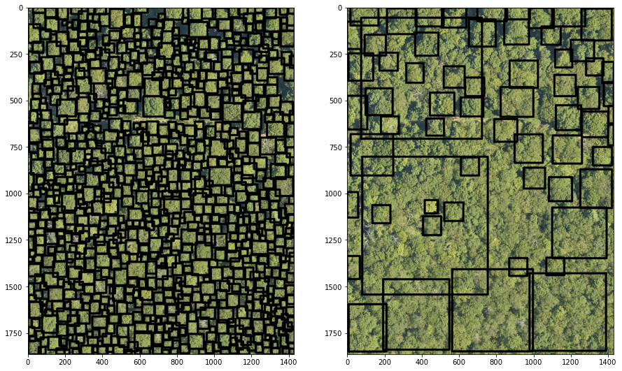
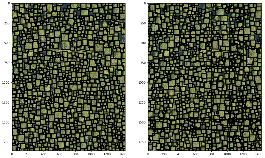
Comparison full image prediction and reference labels
Let’s compare the labels and predictions over the tested image.
fig = plt.figure(figsize=(15,15))
ax1 = plt.subplot(1, 2, 1), cv2_imshow(np.flip(image2,2))
ax2 = plt.subplot(1, 2, 2), cv2_imshow(np.flip(image3,2))
plt.show() # To show figure
Interpretation:
It seems the pretrained model doesn’t perform well with the tested image.
The low performance might be explained due to the pretrained model used 10cm resolution images.
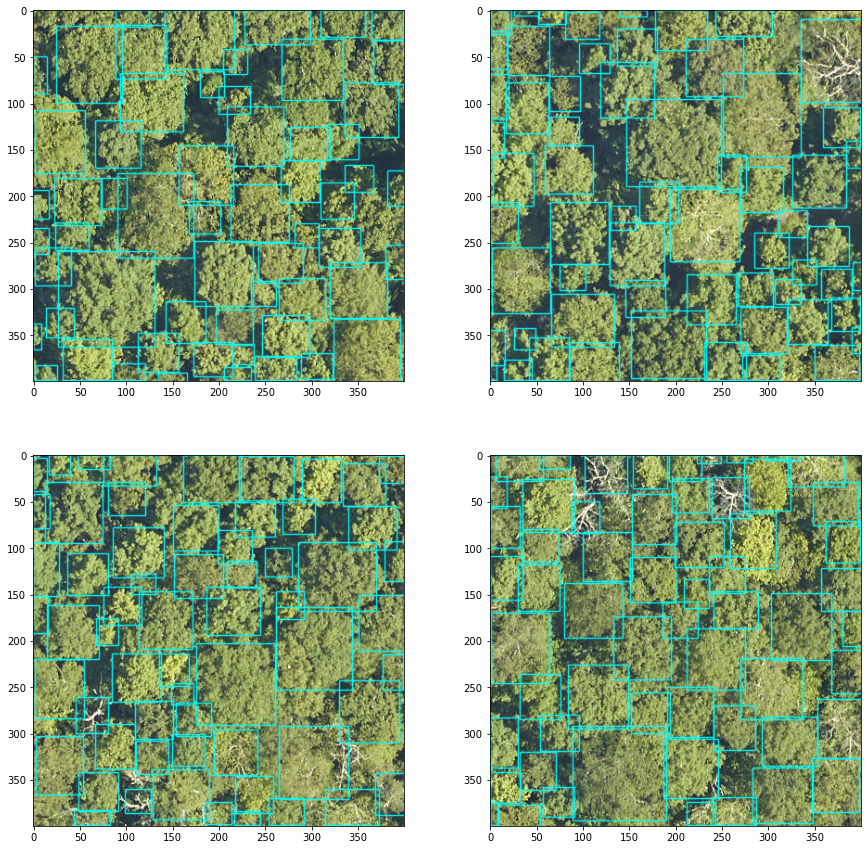
Tile-based prediction
To optimise the predictions, the DeepForest can be run tile-wise.
The following cells show how to define the optimal window i.e. tile size.
from deepforest import preprocess

#Create windows of 400px
windows = preprocess.compute_windows(image.values, patch_size=400,patch_overlap=0)
print(f'We have {len(windows)} in the image')
We have 20 in the image
#Loop through a few sample windows, crop and predict
fig, axes, = plt.subplots(nrows=2,ncols=2, figsize=(15,15))
axes = axes.flatten()
for index2 in range(4):
    crop = image.values[windows[index2].indices()]
    #predict in bgr channel order, color predictions in red.
    boxes = model.predict_image(image=np.flip(crop[...,::-1],2), return_plot = True)

    #but plot in rgb channel order
    axes[index2].imshow(boxes[...,::-1])
/Users/acoca/anaconda3/envs/envai-book/lib/python3.8/site-packages/deepforest/predict.py:32: UserWarning: Image type is {}, transforming to float32. This assumes that the range of pixel values is 0-255, as opposed to 0-1.To suppress this warning, transform image (image.astype('float32')
  warnings.warn("Image type is {}, transforming to float32. This assumes that the range of pixel values is 0-255, as opposed to 0-1.To suppress this warning, transform image (image.astype('float32')")
Once a suitable tile size is defined, we can run in a batch using the predict_tile function:
tile = model.predict_tile(image=image.values,return_plot=False,patch_overlap=0,iou_threshold=0.05,patch_size=400)

# plot predicted bbox
image_tile = image.values.copy()

for index, row in tile.iterrows():
    cv2.rectangle(image_tile, (int(row["xmin"]), int(row["ymin"])), (int(row["xmax"]), int(row["ymax"])), (0, 0, 0), thickness=10, lineType=cv2.LINE_AA)

fig = plt.figure(figsize=(15,15))
ax1 = plt.subplot(1, 2, 1), cv2_imshow(np.flip(image2,2))
ax2 = plt.subplot(1, 2, 2), cv2_imshow(np.flip(image_tile,2))
plt.show() # To show figure
0%| | 0/20 [00:00<?, ?it/s]
5%|██████▊ | 1/20 [00:03<01:08, 3.59s/it]
10%|█████████████▌ | 2/20 [00:07<01:04, 3.56s/it]
15%|████████████████████▍ | 3/20 [00:10<01:00, 3.54s/it]
20%|███████████████████████████▏ | 4/20 [00:14<00:56, 3.55s/it]
25%|██████████████████████████████████ | 5/20 [00:17<00:53, 3.56s/it]
30%|████████████████████████████████████████▊ | 6/20 [00:21<00:49, 3.56s/it]
35%|███████████████████████████████████████████████▌ | 7/20 [00:24<00:46, 3.56s/it]
40%|██████████████████████████████████████████████████████▍ | 8/20 [00:28<00:42, 3.54s/it]
45%|█████████████████████████████████████████████████████████████▏ | 9/20 [00:31<00:37, 3.45s/it]
50%|███████████████████████████████████████████████████████████████████▌ | 10/20 [00:34<00:33, 3.36s/it]
55%|██████████████████████████████████████████████████████████████████████████▎ | 11/20 [00:38<00:30, 3.36s/it]
60%|█████████████████████████████████████████████████████████████████████████████████ | 12/20 [00:41<00:27, 3.41s/it]
65%|███████████████████████████████████████████████████████████████████████████████████████▊ | 13/20 [00:45<00:24, 3.43s/it]
70%|██████████████████████████████████████████████████████████████████████████████████████████████▌ | 14/20 [00:48<00:20, 3.42s/it]
75%|█████████████████████████████████████████████████████████████████████████████████████████████████████▎ | 15/20 [00:52<00:17, 3.50s/it]
80%|████████████████████████████████████████████████████████████████████████████████████████████████████████████ | 16/20 [00:55<00:14, 3.51s/it]
85%|██████████████████████████████████████████████████████████████████████████████████████████████████████████████████▊ | 17/20 [00:59<00:10, 3.51s/it]
90%|█████████████████████████████████████████████████████████████████████████████████████████████████████████████████████████▌ | 18/20 [01:02<00:07, 3.50s/it]
95%|████████████████████████████████████████████████████████████████████████████████████████████████████████████████████████████████▎ | 19/20 [01:06<00:03, 3.50s/it]
100%|███████████████████████████████████████████████████████████████████████████████████████████████████████████████████████████████████████| 20/20 [01:09<00:00, 3.50s/it]
100%|███████████████████████████████████████████████████████████████████████████████████████████████████████████████████████████████████████| 20/20 [01:09<00:00, 3.49s/it]
Interpretation
The tile-based prediction provides more reasonable results than predicting over the whole image.
While the prediction looks closer to the ground truth labels, there seem to be some tiles edges artefacts. This will require further investigation i.e. inspecting the
deepforesttile-wise prediction function to understand how the predictions from different tiles are combined after the model has made them.
Summary
This notebook has demonstrated the use of:
The
deepforestpackage to easily load and run a pretrained model for tree crown classification from very-high resolution RGB imagery.tile-wiseto considerably improve the prediction. However, user should define an optimal tile size.cv2to visualise the bounding box.